Filling#06 - 후니넷

A Simple Example

Just to reiterate the algorithm, the following simple example of scan-line polygon filling will be outlined.

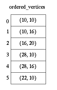
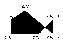
Initially, each vertice of the polygon is given in the form of (x,y) and is in an ordered array as such:

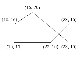
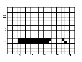
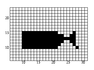
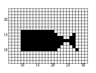
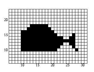
Unfilled, the polygon would look like this to the human eye:

We will now walk through the steps of the algorithm to fill in the polygon.

Initializing All of the Edges:
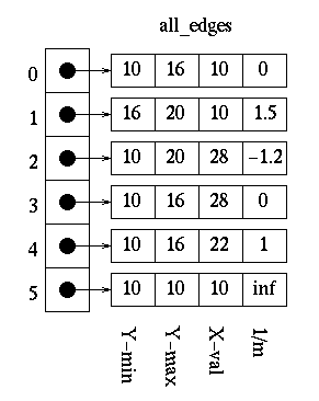
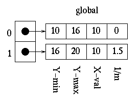
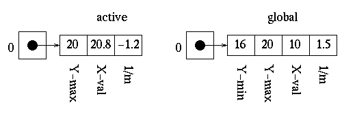
We want to determine the minimum y value, maximum y value, x value, and 1/m for each edge and keep them in the all_edges table. We determine these values for the first edge as follows:
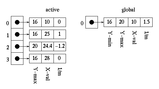
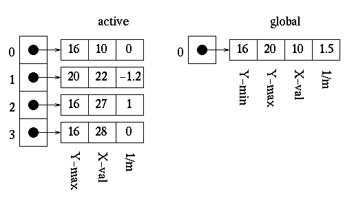
The edge value results are in the form of Y-min, Y-max, X-val, Slope for each edge array pointed to in the all_edges table. As a result of calculating all edge values, we get the following in the all_edges table.
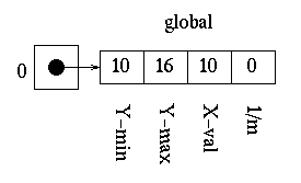
Initializing the Global Edge Table:
We want to place all the edges in the global edge table in increasing y and x values, as long as slope is not equal to zero.

For the first edge, the slope is not zero so it is placed in the global edge table at index=0.

For the second edge, the slope is not zero and the minimum y value is greater than that at zero, so it is placed in the global edge table at index=1.

For the third edge, the slope is not zero and the minimum y value is equal the edge's at index zero and the x value is greater than that at index 0, so the index is increased to 1. Since the third edge has a lesser minimum y value than the edge at index 2 of the global edge table, the index for the third edge is not increased againg. The third edge is placed in the global edge table at index=1.

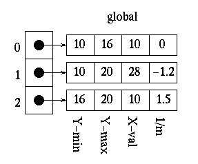
We continue this process until we have the following:

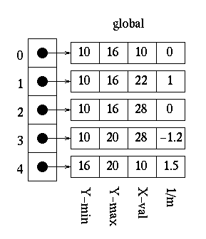
Notice that the global edge table has only five edges and the all_edges table has six. This is due to the fact that the last edge has a slope of zero and, therefore, is not placed in the global edge table.
Initializing Parity
Parity is initially set to even.
Initializing the Scan-Line
Since the lowest y value in the global edge table is 10, we can safely choose 10 as our initial scan-line.
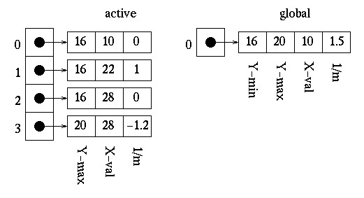
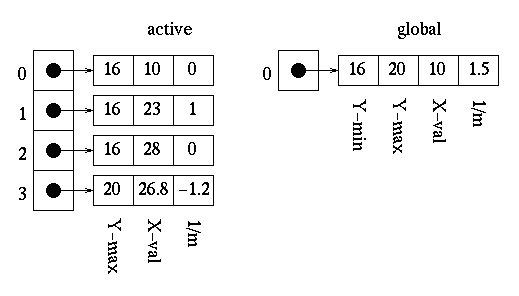
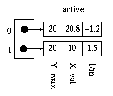
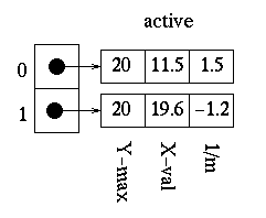
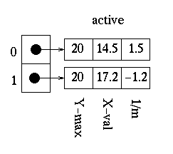
Initializing the Active Edge Table
Since our scan-line value is 10, we choose all edges which have a minimum y value of 10 to move to our active edge table. This results in the following.
Filling the Polygon
Starting at the point (0,10), which is on our scan-line and outside of the polygon, will want to decide which points to draw for each scan-line.
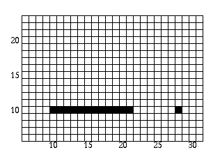
1. Scan-line = 10:
  Once the first edge is encountered at x=10, parity = odd. All points are drawn from this point until the next edge is encountered at x=22. Parity is then changed to even. The next edge is reached at x=28, and the point is drawn once on this scan-line due to the special parity case. We are now done with this scan-line.
  
  First, we update the x values in the active edge table using the formula x₁ = x₀ + 1/m to get the following:
  
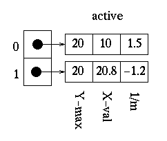
  The edges then need to be reordered since the edge at index 3 of the active edge table has a lesser x value than that of the edge at index 2. Upon reordering, we get:
  
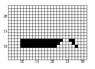
  The polygon is now filled as follows:
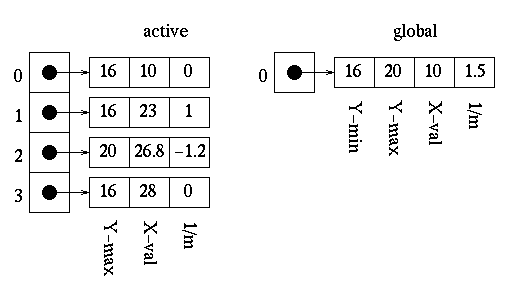
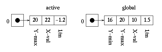
2. Scan-line = 11:
  Once the first edge is encountered at x=10, parity = odd. All points are drawn from this point until the next edge is encountered at x=23. Parity is then changed to even. The next edge is reached at x=27 and parity is changed to odd. The points are then drawn until the next edge is reached at x=28. We are now done with this scan-line.
  
  Upon updating the x values, the edge tables are as follows:
  
  It can be seen that no reordering of edges is needed at this time.
  
  The polygon is now filled as follows:
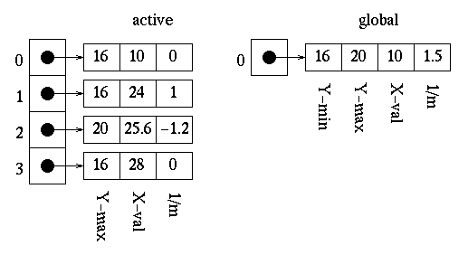
3. Scan-line = 12:
  Once the first edge is encountered at x=10, parity = odd. All points are drawn from this point until the next edge is encountered at x=24. Parity is then changed to even. The next edge is reached at x=26 and parity is changed to odd. The points are then drawn until the next edge is reached at x=28. We are now done with this scan-line.
  
  Updating the x values in the active edge table gives us:
  
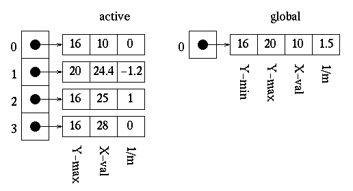
  We can see that the active edges need to be reordered since the x value of 24.4 at index 2 is less than the x value of 25 at index 1. Reording produces the following:
  
  The polygon is now filled as follows:
4. Scan-line = 13:
  Once the first edge is encountered at x=10, parity = odd. All points are drawn from this point until the next edge is encountered at x=25 Parity is then changed to even. The next edge is reached at x=25 and parity is changed to odd. The points are then drawn until the next edge is reached at x=28. We are now done with this scan-line.
  
  Upon updating the x values for the active edge table, we can see that the edges do not need to be reordered.
  
  The polygon is now filled as follows:
5. Scan-line = 14:
  Once the first edge is encountered at x=10, parity = odd. All points are drawn from this point until the next edge is encountered at x=24. Parity is then changed to even. The next edge is reached at x=26 and parity is changed to odd. The points are then drawn until the next edge is reached at x=28. We are now done with this scan-line.
  
  Upon updating the x values for the active edge table, we can see that the edges still do not need to be reordered.
  
  The polygon is now filled as follows:
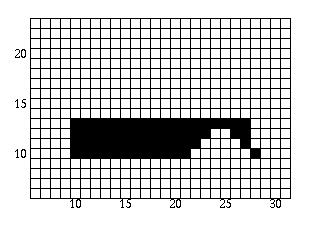
6. Scan-line = 15:
  Once the first edge is encountered at x=10, parity = odd. All points are drawn from this point until the next edge is encountered at x=22. Parity is then changed to even. The next edge is reached at x=27 and parity is changed to odd. The points are then drawn until the next edge is reached at x=28. We are now done with this scan-line.
  
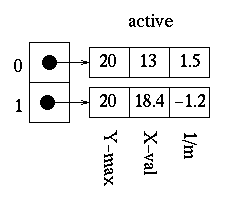
  Since the maximum y value is equal to the next scan-line for the edges at indices 0, 2, and 3, we remove them from the active edge table. This leaves us with the following:
  
  We then need to update the x values for all remaining edges.
  
  Now we can add the last edge from the global edge table to the active edge table since its minimum y value is equal to the next scan-line. The active edge table now look as follows (the global edge table is now empty):
  
  These edges obviously need to be reordered. After reordering, the active edge table contains the following:
  
  The polygon is now filled as follows:
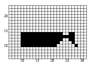
7. Scan-line = 16:
  Once the first edge is encountered at x=10, parity = odd. All points are drawn from this point until the next edge is reached at x=21. We are now done with this scan-line. The x values are updated and the following is obtained:
  
  The polygon is now filled as follows:
8. Scan-line = 17:
  Once the first edge is encountered at x=12, parity = odd. All points are drawn from this point until the next edge is reached at x=20. We are now done with this scan-line. We update the x values and obtain:
  
  The polygon is now filled as follows:
9. Scan-line = 18:
  Once the first edge is encountered at x=13, parity = odd. All points are drawn from this point until the next edge is reached at x=19. We are now done with this scan-line. Upon updating the x values we get:
  
  The polygon is now filled as follows:
10. Scan-line = 19:
  Once the first edge is encountered at x=15, parity = odd. All points are drawn from this point until the next edge is reached at x=18. We are now done with this scan-line. Since the maximum y value for both edges in the active edge table is equal to the next scan-line, we remove them. The active edge table is now empty and we are now done.
  
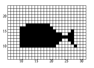
  The polygon is now filled as follows:
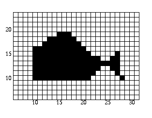
Now that we have filled the polygon, let's see what it looks like to the naked eye:

Do You Understand The Algorithm?

Hopefully, by now you have at least a basic understanding of the scan-line polygon fill algorithm. If you are unsure, try the demo below.

Above, you will find a scan-line polygon fill demo. You may wish to use a piece of paper and/or calculator to do the calculations.

The demo automatically initializes the global edge table, scan-line, and active edge table for the following ordered list of points:

Point( 1, 1 )
Point( 1, 6 )
Point( 9, 14 )
Point( 3, 14 )
Point( 9, 8 )
Point( 5, 4 )
Point( 11, 4 )
Point( 11, 10 )
Point( 14, 10 )
Point( 14, 1 )

Here's what needs to be done for each scan-line:

For each scan-line, start by selecting the next pixel to be filled by clicking on it with the mouse. If you select the incorrect pixel, a message will appear at the bottom of the window prompting you to select another.
Once all of the pixels for the scan-line have been filled in, increment the scan-line by clicking on the Scan-line button.
Next, click on the Remove Edges From AET button to check for and remove any edges from the active edge table for which the scan-line is equal to the maximum y value.
Select the Update X Values button to update the x values in the active edge table for the current scan-line.
If there are any edges left in the global edge table, select the Add Edges To AET button to check for any edges in the global edge table for which the minimum y value is equal to the current scan-line and add them to the active edge table.
Select the Reorder AET button to reorder the edges in the active edge table.
If the active edge table still contains edges, start again at step 1 for the current scan-line.

If, at any time, you wish to restart the demo, select the Restart button with the mouse.

You will receive a score upon completion. If you are not happy with your score and are still a bit confused, you may want to review this teaching tool again or take a look at some additional resources. Otherwise, congratulations! You are now on your way to implementing a scan-line polygon fill.

<< Previous Page

Next Page >>

Contents

A Simple Example

Do You Understand The Algorithm?

로그인